The Ultimate Tutorial on Splitting Your Excel Window for Enhanced Productivity

Quick Links

• Using the Split Screen Function
• Creating Four Equal Quadrants
• Vertical and Horizontal Splits

Splitting screens, whether vertically or horizontally, is a great way to streamline your workflow when using Excel. Using this feature lets you simultaneously view separate sections of a spreadsheet, enabling you to compare data quickly. Here’s how.

Using the Split Screen Function

If you have a spreadsheet packed with data, navigating it can be quite cumbersome, especially if you want to compare data from several different sections of the spreadsheet. Taking advantage of Excel’s split-screen functionality can streamline this process. Excel also lets you customize how the screen is split, giving you complete control for your specific needs.

Finding the split screen function is easy enough. Just head over to the “View” tab and click the “Split” option.

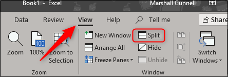
That said, there are a few ways to use this feature to split the screen.

Creating Four Equal Quadrants

Excel lets you split the screen into four equal quadrants. This gives you four copies of your current worksheet, all on the same screen! To do this, first, make sure that you’ve got the A1 cell selected.

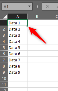
Next, head back over to the “View” tab and click the “Split” button. This will split your screen into four equal worksheets.

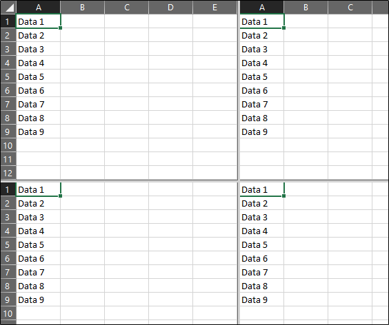
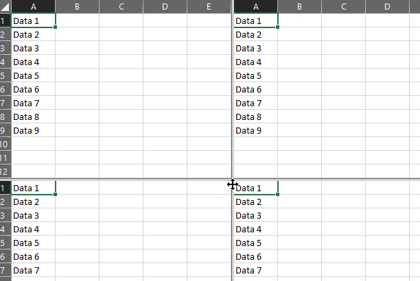
You can also tweak where the split is by clicking and dragging either side of one of the worksheets, or the center section.

Vertical and Horizontal Splits

If you don’t need four copies of the worksheet, you can split the screen in two instead. You can split the screen horizontally or vertically, depending on what you need.

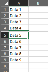
To split the screen horizontally, select a cell from column A in any row (Except for the A1 cell). Next, click the “Split” button on the “View” tab. The split will appear above the selected row. For example, if we select cell A5, the split will look like this:

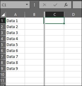
Splitting the screen vertically is just as easy. Select a cell from any column (except column A) in row 1 and click the “Split” button.

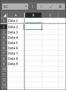
You don’t have to follow these rules exactly. Selecting any cell from any row will split the spreadsheet. The only thing to remember is that, unless you select a cell from the first row or from column A, the screen will be split into four instead of two.

Once you’re finished with the feature and are ready to get the screen back to a single worksheet, simply click the “Split” option again to turn it off. Alternatively, you can drag the sides of the split screen bars to the edge of the window to disable the feature.