Mastering Uniqueness: A Guide to Identifying and Organizing Distinct Data with Microsoft Excel

Quick Links

When you want a list of customers, email addresses, product IDs, or something similar where each one is distinct, Excel has a function to help. We’ll show you how to use this function to list unique values and text.

You can already use functions in Excel to total the number of distinct values . But here we’ll show you how to list those values instead using the UNIQUE function. Plus, we’ll throw in easy ways to sort the list and combine values.

As of March 2022, the UNIQUE function is available in Excel for Microsoft 365, Excel for the web, Excel 2021 or later, or Excel for iPhone, iPad, or Android phones or tablets.

Use the UNIQUE Function in Excel

You can use the UNIQUE function for text or numbers, decide how to compare the cell range, and opt to show results that only appear once.

The syntax for the function is

    `UNIQUE(array, column, only_once)`

where only the first argument is required. Include the

    `column`

argument to compare columns instead of rows and the only_once argument to return values that occur only one time in the array.

Should you choose to include the optional arguments, you’ll use the TRUE indicator in the formula for each. If no indicator is included, the function assumes FALSE.

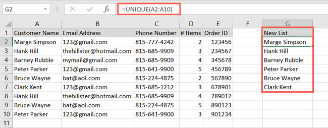
As an example, we’ll create a list of customers for an email blast. Rather than use the existing list in cells A2 through A10 because some customers ordered more than once, we’ll make a new list where each customer appears one time.

=UNIQUE(A2:A10)

For another example, we’ll add the third argument, only_once, to find those customers who’ve only ordered once.

=UNIQUE(A2:A10,,TRUE)

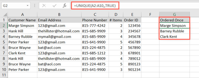
Because the second argument assumes FALSE if nothing is included, we simply add a comma after the first argument and then another comma before the last argument. Alternatively, you can use this formula to obtain the same result:

=UNIQUE(A2:A10,FALSE,TRUE)

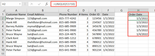
You can use the UNIQUE function to list distinct values as well as text. In this formula, we can list unique dates :

=UNIQUE(F2:F10)

Sort the List Automatically

As mentioned, you can sort the list automatically at the same time you use the UNIQUE function to create it. To do this, you simply add the SORT function to the beginning of the formula.

The SORT function is currently only available in the Excel versions listed earlier .

The syntax for this function is SORT(array, index, order, column) where only the first argument is required.

Using the first list of unique customers we created above and sort it immediately, you would use this formula:

=SORT(UNIQUE(A2:A10))

As you can see, the UNIQUE formula is the required array argument for the SORT function.

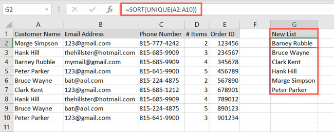
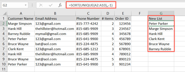
By default, the SORT function lists items in ascending order. To sort the same list in descending order, you would use the following formula which adds the order argument.

=SORT(UNIQUE(A2:A10),,-1)

Notice here we have a double comma again. This is because we don’t want the index argument, only the order argument. Use 1 for ascending order and -1 for descending order. If no value is used, the function assumes 1 by default.

Combine Unique Values

One more handy addition to the UNIQUE function allows you to combine values. For instance, maybe your list has values in two columns instead of just one as in the screenshot below.

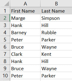
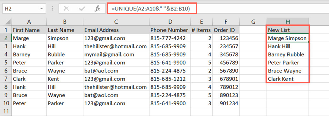
By adding the ampersand (&) operator and a space, we can create a list of first and last names of unique customers with this formula:

=UNIQUE(A2:A10&” “&B2:B10)

To break down the formula, the first array, A2 through A10, contains the first names, the ampersands concatenate the first names to the last names in B2 through B10 with a space between them in quotes.

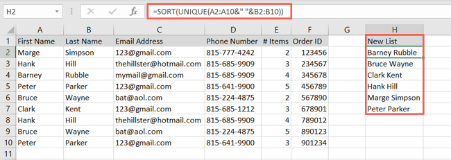
You can also include the SORT function here to put your list in ascending order with this formula:

=SORT(UNIQUE(A2:A10&” “&B2:B10))

Just like you might want to highlight duplicate values in Excel , you may want to find unique ones. Keep the UNIQUE function and these additional ways to use it in the mind the next time you need to create a list of distinct values or text in Excel.

Win Howtos

Mastering Uniqueness: A Guide to Identifying and Organizing Distinct Data with Microsoft Excel