Mastering Precision with Excel’s TRUNCATE Feature: A Step-by-Step Guide

Quick Links

• What Is the TRUNC Function?
• How to Use the TRUNC Function
• Remove the Time from a Date-Time Stamp
• Use TRUNC to Shorten Numbers

There are a variety of ways in Excel to remove decimal points and shortening number values. In this article, we explain how to use the TRUNC function and what makes it different from other techniques.

What Is the TRUNC Function?

The TRUNC function truncates a number to a specified number of decimal places. The key factor that makes TRUNC different from other functions that remove decimal places is that the TRUNC function does not round values. If you use TRUNC to remove all the decimals from the value 4.68, the result is 4.

The TRUNC function requires two pieces of information:

=TRUNC(number, [digits])

The number is the value you want to truncate. Digits are the number of numerals you want to truncate the value to. The digits portion is optional, and if not answered, TRUNC will remove all decimal places.

How to Use the TRUNC Function

Let’s look at examples of the TRUNC function with some sample data. The below example uses the following TRUNC function.

=TRUNC(A2)

If you do not specify how many digits to truncate, all decimal places will be removed.

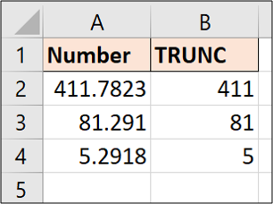
You can see with the value in cell A2 that the TRUNC function does not apply any rounding. It simply truncates the number to 411.

Let’s see another example. This time we will reduce the values to two decimal places.

=TRUNC(A2,2)

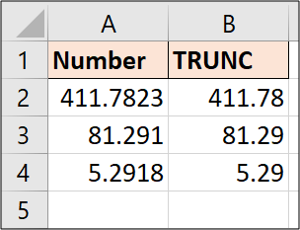
The TRUNC function will not display extra decimals if you ask it to show more than you have.

Take the following example, and let’s truncate it to two decimal places.

=TRUNC(A2,2)

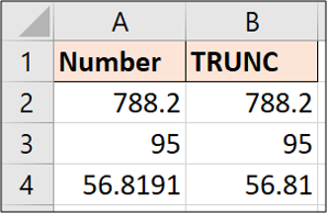
The value in cell A4 is reduced to two decimal places, but the values in A2 and A3 stay as they are because they have less than two decimal places already.

If you want to display the two decimals, the cells will need to be formatted to be forced to show them.

Remove the Time from a Date-Time Stamp

A useful example of TRUNC is to remove the time from a date and time stamp in Excel.

Imagine having the following date and time stamps, but we just want the date in a column for analysis.

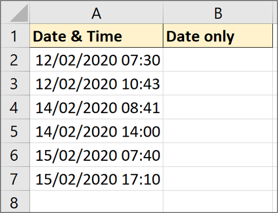
The following formula will work to remove the time.

=TRUNC(A2)

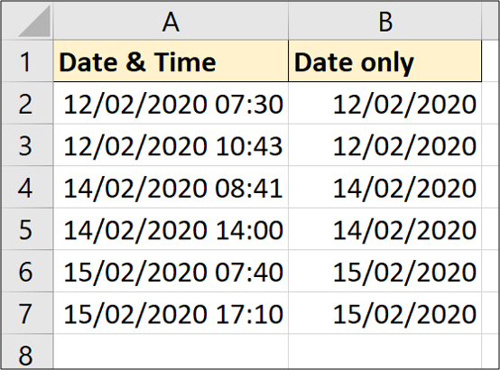
Although the time is removed, the resulting cells will still need to be formatted as a date only.

Use TRUNC to Shorten Numbers

This is a rare technique, but it is worth knowing that the TRUNC function will also accept negative numbers for the digits argument. When you use a negative number, the formula truncates the numbers to the left of the decimal point. However, it does not change the number of digits. It will replace them with zeroes.

Let’s look at the following example.

=TRUNC(A2,-1)

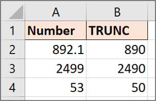
You can see in each example that zero was used to replace the number that was removed from the left of the decimal point.

There are multiple ways in Excel to remove decimal places, however, most of these will apply a rounding of some nature. The strength of the TRUNC function is that it does not round values and simply shortens them to the specified decimal place amount.