Mastering Data Analysis: Building a Pivot Table Using Microsoft Excel's Features

Mastering Data Analysis: Building a Pivot Table Using Microsoft Excel’s Features

Quick Links

If you’re like many spreadsheet application users, you might feel intimidated by pivot tables. But if you start with the basics and learn how to build a pivot table in Microsoft Excel, it can become your favorite feature.

What Are PivotTables in Excel?

A pivot table provides an interactive way for you to arrange, group, calculate, and analyze data. You can manipulate the same data several different ways to view exactly what you need. Pivot tables give you a robust way to work with a data set to spot patterns, review summaries, and calculate counts, averages, or totals.

You would normally create a pivot table if you have an extensive amount of data. This is what makes the pivot table a valuable tool; its ability to make large amounts of data more manageable for analysis .

Microsoft uses “PivotTables” as a single word in its documentation and interfaces surrounding “pivot tables.” So, you may see both terms as you use the application, and we’ll include both in this tutorial as applicable.

Greeting Card Builder

Make a Basic Pivot Table in Excel

To get started, select your data . You can create a pivot table from a range of cells or an existing table structure. Just make sure that you have a row of headers at the top and no empty columns or rows.

You then have two ways to make the pivot table. You can use one of Excel’s recommended PivotTables or create the table yourself.

Use a Recommended PivotTable

Just like inserting a graph in Excel with the recommended chart options, you can do the same with a pivot table. Excel then reviews your data for tables that fit.

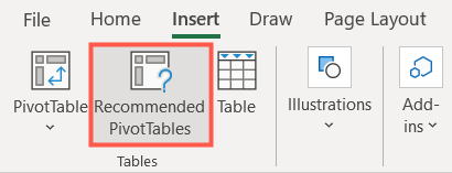
Go to the Insert tab and click “Recommended PivotTables” on the left side of the ribbon.

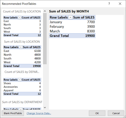
When the window opens, you’ll see several pivot tables on the left. Select one to see a preview on the right. If you see one you want to use, choose it and click “OK.”

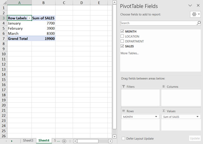
A new sheet will open with the pivot table you picked. You’ll also see the PivotTable Fields sidebar on the right which allows you to edit the table, which we explain below.

KoolReport Pro is an advanced solution for creating data reports and dashboards in PHP. Equipped with all extended packages , KoolReport Pro is able to connect to various datasources, perform advanced data analysis, construct stunning charts and graphs and export your beautiful work to PDF, Excel, JPG or other formats. Plus, it includes powerful built-in reports such as pivot report and drill-down report which will save your time in building ones.

It will help you to write dynamic data reports easily, to construct intuitive dashboards or to build a whole business intelligence cockpit.

KoolReport Pro package goes with Full Source Code, Royal Free, ONE (1) Year Priority Support, ONE (1) Year Free Upgrade and 30-Days Money Back Guarantee.

Developer License allows Single Developer to create Unlimited Reports, deploy on Unlimited Servers and able deliver the work to Unlimited Clients.

Make Your Own Pivot Table

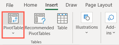
If you want to dive right in and create your own pivot table instead, go to the Insert tab and pick “PivotTable” in the ribbon.

You’ll see a window appear for PivotTable From Table or Range. At the top, confirm the data set in the Table/Range box. Then, decide if you want the table in a new worksheet or your existing one. For analyzing multiple tables, you can check the box to add it to the Data Model. Click “OK.”

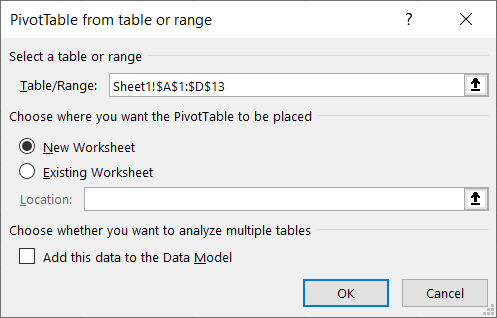
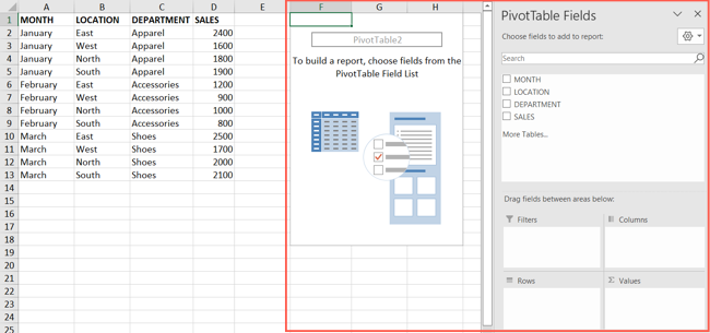
You’ll then see the pivot table and the PivotTable Fields sidebar, ready for you to build your table or edit the recommended table you inserted.

Build or Edit the Pivot Table

Using the PivotTable Fields sidebar, start by choosing the fields at the top you want to include by checking the boxes.

You can check and uncheck boxes for the fields you want to use at any time.

Excel then drops those fields into the boxes at the bottom of the sidebar where it believes they belong. This is where you will decide how you want to place them in your table.

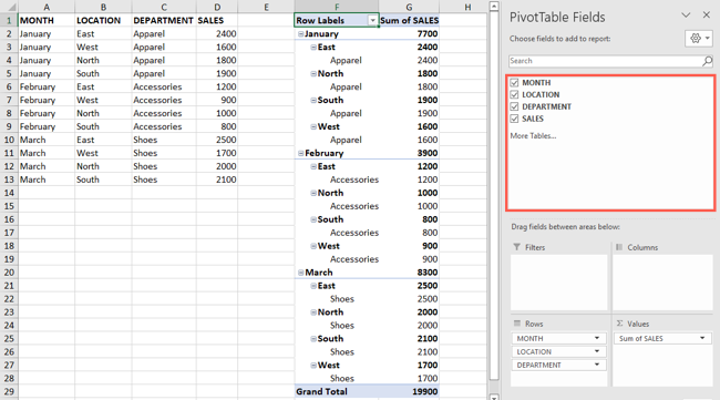
Depending on the type of data in your sheet, you’ll see things like numbers in the Values box, dates and times in the Columns box, and textual data in the Rows box. These are the defaults for those types of data, but you can move them where you want them.

As an example, we want to see our Months as columns instead of rows. You simply drag that field from the Rows box to the Columns box and your table will update accordingly. Alternatively, you can use the drop-down arrows next to the fields to move them.

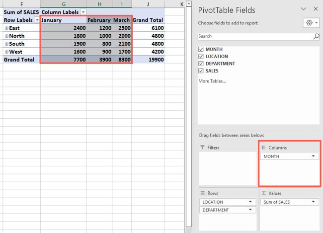
If you have more than one field in a box, the order determines the placement in the pivot table as well. In this example, we have Department first and Location second in the Rows box which is how they’re grouped in the table.

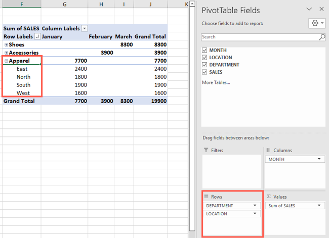
But by moving Location above Department, we see each of our locations as the main fields instead, which is what we want. Then, we simply use the minus and plus buttons next to each Location to expand the group and view the Departments.

Because you can move the fields between the boxes with simple drag-and-drop actions, this allows you to easily find the best fit for your data analysis .

Filter or Sort the Pivot Table

The perks of using a table in Excel include the ability to filter and sort your data as needed. Pivot tables offer these same functions.

You’ll see filters built-in for your first column and depending on your data arrangement, maybe more than one column. To apply a filter to the column, click the filter button next to the header and choose how to filter the data as you normally would in an Excel table.

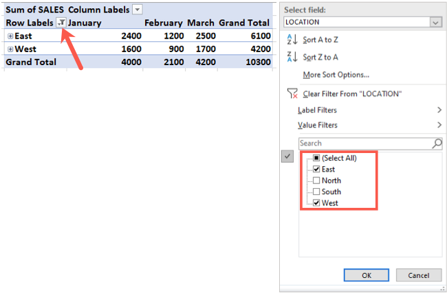
To sort, click the button and select a sort option.

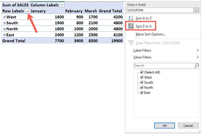
Any DRM Removal for Win：Remove DRM from Adobe, Kindle, Sony eReader, Kobo, etc, read your ebooks anywhere.

Add a Table Filter

You can also apply a filter to the top level of the table. Using our example, we want to filter the entire table to see each Department, one at a time. Drag the field you want to use as the filter into the Filters box in the PivotTable Fields sidebar.

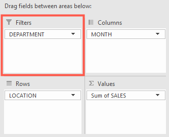
You’ll see your table update to place this filter at the top. Then, click the filter button to apply the one you want at the time.

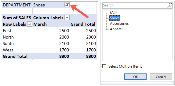
To remove this higher-level table filter, simply drag the field out of the Filter box in the sidebar.

Well, there you have it! The bare-bones basics you need to create a pivot table in Excel. Hopefully this how-to gets you off to a great start with your own pivot table!

Win Howtos