Mastering Cell Style Formatting: A Comprehensive Guide to Customizing Your Excel Spreadsheets

Quick Links

• Apply a Premade Cell Style in Excel
• Create a Custom Cell Style in Excel
• Remove a Cell Style

There are many ways to format your Excel spreadsheets. From automatic conditional formatting to simple copying from another cell , we take shortcuts to format our sheets quickly. Another wonderful feature for formatting in Microsoft Excel is a Cell Style.

Cell styles in Excel combine multiple formats. For instance, you might have a yellow fill color, a bold font, a number format, and a cell border all in a single style. This allows you to quickly apply multiple formats to the cells while adding consistency to the appearance of your sheet.

Apply a Premade Cell Style in Excel

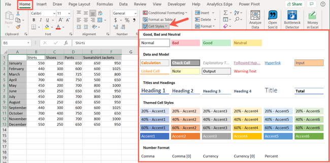
Excel does a good job of offering many premade cell styles that you can use. These cover everything from titles and headings to colors and accents to currency and number formats.

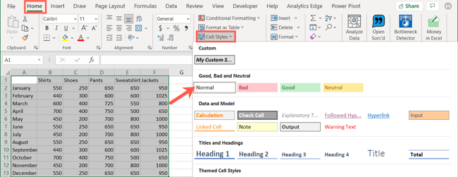
To view and apply a cell style, start by selecting a cell or range of cells. Go to the Home tab and click “Cell Styles” in the Styles section of the ribbon. Click any style to apply it to your cell(s).

Create a Custom Cell Style in Excel

While there are plenty of built-in cell styles to pick from, you might prefer to create your own. This lets you choose the exact formats that you want to use, and then reuse that cell style with ease.

Head to the Home tab, click “Cell Styles,” and choose “New Cell Style.”

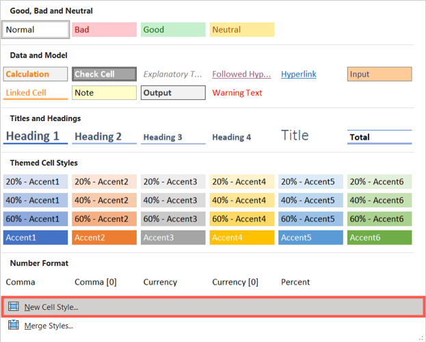
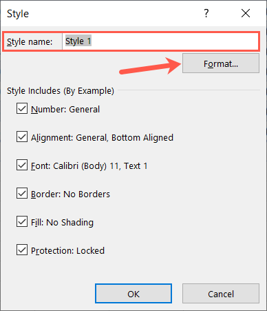
Give your custom style a name at the top of the Style box. Then, click “Format.”

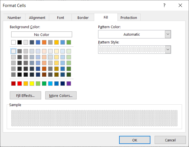
In the Format Cells window, use the various tabs to select the styles for number, font, border, and fill as you want them to apply. As an example, we’ll create My Custom Style and use a currency number format , bold and italic font, an outline border, and a gray, dotted fill pattern.

After choosing the formats that you want, click “OK,” which returns you to the Style window.

In the Style Includes section, you’ll see the formats that you just picked. Uncheck any formats that you don’t want to use and click “OK” when you finish.

Power Tools add-on for Google Sheets, 12-month subscription

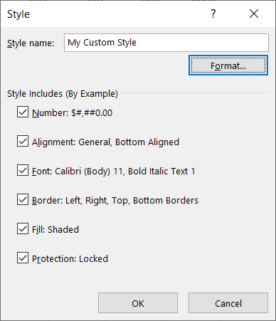
To use your custom cell style, select the cells, go to the Home tab, and click “Cell Styles.” You should see your newly created style at the top of the selection box under Custom. Click to apply it to your cells.

A cell style that you create is available in all your spreadsheets, but only in the Excel workbook where you create it.

Edit a Cell Style

If you want to make changes to a custom cell style that you created or even to a premade style, head back to the Home tab. Click “Cell Styles,” right-click the style that you want to edit, and pick “Modify.”

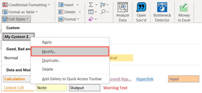
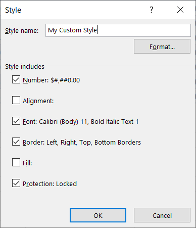
When the Style window opens, click “Format” to make your adjustments in the Format Cells window, and then click “OK.” Make any further changes in the Style window, such as inputting a new name if you’re modifying a premade style, and then click “OK” there as well.

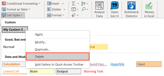
You can also delete a custom style that you created by choosing “Delete” instead of “Modify” in the shortcut menu.

When you’ve perfected your custom look, it’s easy to share cell styles across workbooks .

Remove a Cell Style

If you decide later on to remove a cell style that you applied, it only takes a few clicks to do so.

Select the cell(s) and go back to the Home tab. Click “Cell Styles” and choose “Normal” near the top under Good, Bad, and Neutral.

OtsAV Radio Webcaster

Make your spreadsheet’s appearance attractive and consistent with premade or custom cell styles in Microsoft Excel!

Related: How to Cross Reference Cells Between Microsoft Excel Spreadsheets