Guide: Removing or Masking Erroneous Data Points and Warnings in Microsoft Excel Tables

Quick Links

• Hide Errors with the IFERROR Function
• Background Error Checking
• Turn Off the Excel Error Checking

Your Excel formulas can occasionally produce errors that don’t need fixing. However, these errors can look untidy and, more importantly, stop other formulas or Excel features from working correctly. Fortunately, there are ways to hide these error values.

Hide Errors with the IFERROR Function

The easiest way to hide error values on your spreadsheet is with the IFERROR function. Using the IFERROR function, you can replace the error that’s shown with another value, or even an alternative formula.

In this example, a VLOOKUP function has returned the #N/A error value.

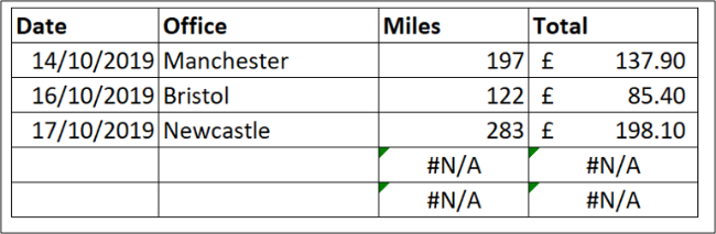
This error is due to there not being an office to look for. A logical reason, but this error is causing problems with the total calculation.

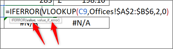
The IFERROR function can handle any error value including #REF!, #VALUE!, #DIV/0!, and more. It requires the value to check for an error and what action to perform instead of the error if found.

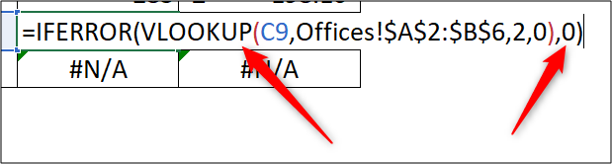
In this example, the VLOOKUP function is the value to check and “0” is displayed instead of the error.

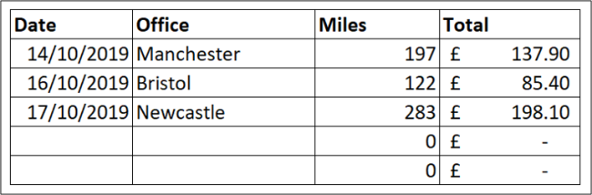
Using “0” instead of the error value ensures the other calculations and potentially other features, such as charts, all work correctly.

Background Error Checking

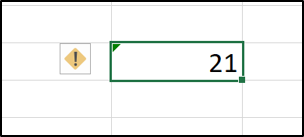
If Excel suspects an error in your formula, a small green triangle appears in the top-left corner of the cell.

Note that this indicator does not mean that there is definitely an error, but that Excel is querying the formula you’re using.

Excel automatically performs a variety of checks in the background. If your formula fails one of these checks, the green indicator appears.

When you click on the cell, an icon appears warning you of the potential error in your formula.

Click the icon to see different options for handling the supposed error.

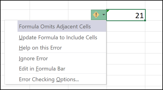
In this example, the indicator has appeared because the formula has omitted adjacent cells. The list provides options to include the omitted cells, ignore the error, find more information, and also change the error check options.

To remove the indicator, you need to either fix the error by clicking “Update Formula to Include Cells” or ignore it if the formula is correct.

Turn Off the Excel Error Checking

If you do not want Excel to warn you of these potential errors, you can turn them off.

Click File > Options. Next, select the “Formulas” category. Uncheck the “Enable Background Error Checking” box to disable all background error checking.

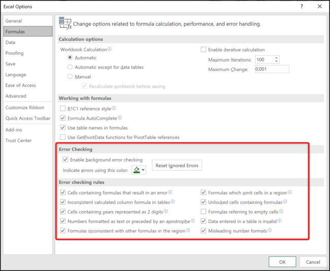
Alternatively, you can disable specific error checks from the “Error Checking Rules” section at the bottom of the window.

By default, all of the error checks are enabled except “Formulas Referring to Empty Cells.”

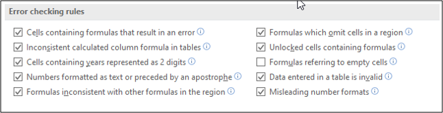
More information about each rule can be accessed by positioning the mouse over the information icon.

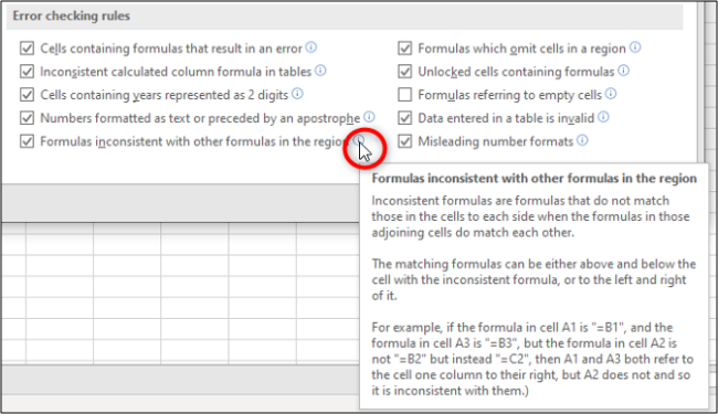
Check and uncheck the boxes to specify which rules you would like Excel to use with the background error checking.

When formula errors do not need fixing, their error values should be hidden or replaced with a more useful value.

Excel also performs background error checking and queries mistakes it thinks you’ve made with your formulas. This is useful but specific or all error checking rules can be disabled if they interfere too much.

Also read: