Excel Essentials: Unlocking Data Management with Advanced Filter Techniques

Quick Links

• What Is the FILTER Function in Excel?
• How to Create a Basic Filter Formula
• Filter Using Multiple Criteria in the FILTER Function
• How to Sort Your Filtered Data in Excel

Key Takeaways

To use the FILTER function, enter simply enter the array and range for your criteria. To avoid an Excel error for empty filter results, use the third optional argument to display a custom indicator.

Microsoft Excel offers a built-in filter feature along with the option to use an advanced filter. But if you want to filter by multiple criteria and even sort the results , check out the FILTER function in Excel.

Using the FILTER function, you can use operators for “and” and “or” to combine criteria. As a bonus, we’ll show you how to apply the SORT function to the formula to display your results in ascending or descending order by a particular column.

What Is the FILTER Function in Excel?

The syntax for the formula is

    `FILTER(array, range=criteria, if_empty)`

where only the first two arguments are required. You can use a cell reference, number, or text in quotes for the criteria, depending on your data.

Use the third optional argument if your data set may return an empty result since it’ll display the #CALC! error by default. To replace the error message, you can include text, a letter, or number in quotes or simply leave the quotes empty for a blank cell.

How to Create a Basic Filter Formula

To get started, we’ll start with a basic filter so that you can see how the function works . In each screenshot, you’ll see our filter results on the right.

Related: How to Find the Function You Need in Microsoft Excel

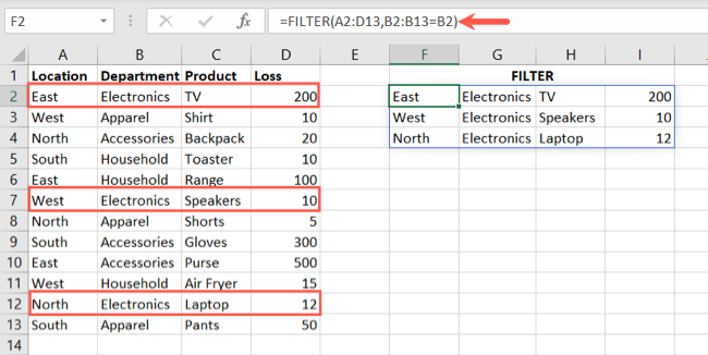
For filtering the data in cells A2 through D13 using the content of cell B2 (Electronics) as criteria, here’s the formula:

=FILTER(A2:D13,B2:B13=B2)

To break down the formula, you see the array argument is A2:D13 and the range=criteria argument is B2:B13=B2. This returns all results containing Electronics.

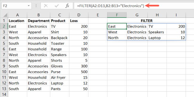
Another way to write the formula is by entering the contents of cell B2 in quotation marks as follows:

=FILTER(A2:D13,B2:B13=”Electronics”)

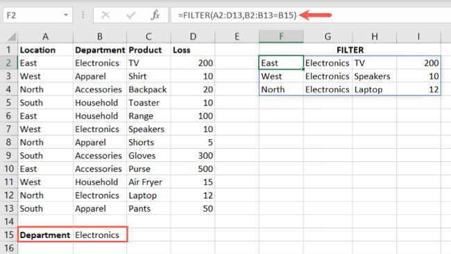
You can also use criteria from another cell to filter the data in the range=criteria area. Here, we’ll use the data in cell B15.

=FILTER(A2:D13,B2:B13=B15)

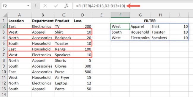
If your data contains a number, you can use this as the criteria without quotation marks. In this example, we’ll use the same cell range, but filter by cells D2 through D13 looking for 10.

=FILTER(A2:D13,D2:D13=10)

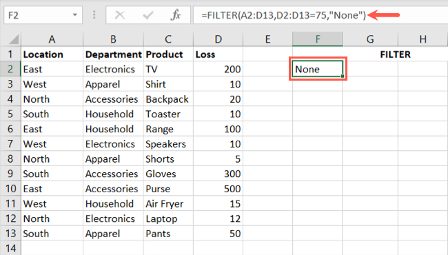
If you aren’t receiving any results for your formula or are seeing the #CALC! error, you can use the third argument if_empty. For instance, we’ll display None if the result is blank.

=FILTER(A2:D13,D2:D13=75,”None”)

As you can see, the range=criteria data doesn’t include 75, therefore, our result is None.

NeoDownloader - Fast and fully automatic image/video/music downloader.

Filter Using Multiple Criteria in the FILTER Function

An advantage of the FILTER function in Excel is that you can filter by multiple criteria. You’ll include an operator for AND (*) or OR (+) .

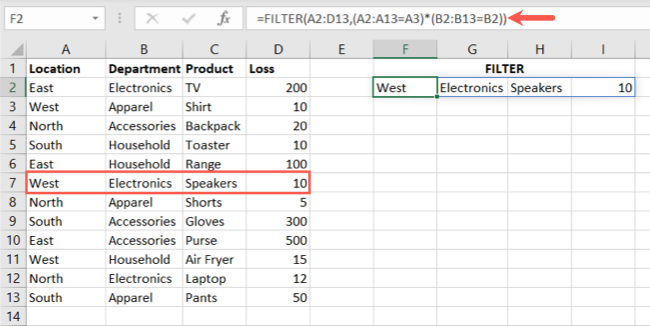
For example, we’ll filter our data set by both A3 (West) and B2 (Electronics) using an asterisk (*) with this formula:

=FILTER(A2:D13,(A2:A13=A3)*(B2:B13=B2))

As you can see, we have one result that includes both West and Electronics.

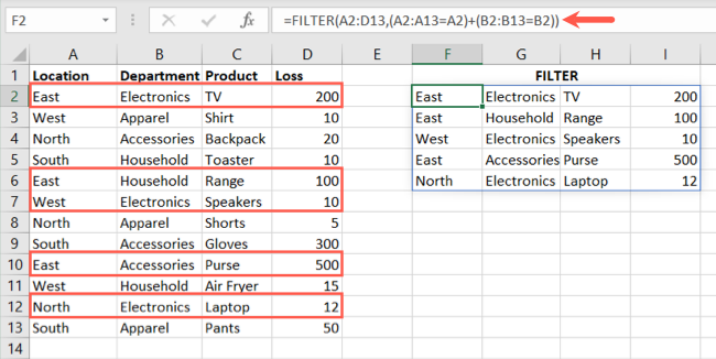
To use the other operator, we’ll filter for either A3 or B2 using a plus sign (+) as follows:

=FILTER(A2:D13,(A2:A13=A3)+(B2:B13=B2))

Now, you can see that our results contain five records with West or Electronics.

How to Sort Your Filtered Data in Excel

If you want to sort the results you receive from the FILTER function, you can add the SORT function to the formula. This is simply an alternative to using the Sort feature on the Data tab, but doesn’t require you to reposition your data.

For more information on the SORT function before you try it out, take a look at our how-to for full details.

Related: How to Use the Microsoft Excel SORT Function

Here, we’ll use our basic filter from the beginning of this tutorial: FILTER(A2:D13,B2:B13=B2). Then, we’ll add SORT with its arguments to sort by the fourth column (Loss) in descending order (-1):

=SORT(FILTER(A2:D13,B2:B13=B2),4,-1)

To break down this formula, we have our FILTER formula as the array argument for the SORT function. After that, we have 4 to sort by the fourth column in the data set and -1 to display the results in descending order.

To display the results in ascending order instead, replace the -1 with 1:

=SORT(FILTER(A2:D13,B2:B13=B2),4,1)

Excel’s built-in filter is great for quickly seeing specific records in a data set. And the advanced filter works well for filtering by a criteria range in place or another location. But for using multiple criteria and sorting at the same time, take the FILTER function for a spin.

| | Mastering Excel Functions | | |
| —————————- | —————————————————————————————————————————————————————————————————————————————————————————————————————————————————————————————————————————————————————————————————————————————————————————————————————————————————————————————————————————————————————————————————————————————————————————————————————————————————————————————————————————————————————————————————————————————————————————————————————————————————————————————————————————————————————————————————————————————————————————————————————————————————————————————————————————————————————————————————————————————————————————————————————————————————————————————————————————————————————————————————————————————————————————————————————————————————————————————————————————————————————————————————————————————————————————————————————————————————————————————————————————————————————————————————————————————————————————————————————————————————————————————————————————————————————————————————————————————————————————————————————————————————————————————————————— | |
| Functions | AVERAGE · CONCATENATE · COUNT · COUNTIF · DATEDIF · FILTER · FREQUENCY · FV · HYPERLINK · IF · IFS · IMAGE · INDEX · IS · LEN · MATCH ·MEDIAN · RAND · ROUND · RRI · SORT · SQRT · SUBSTITUTE · SUBTOTAL · SUM · SUMIF · TODAY · TRIM · TRUNC · VLOOKUP · WEEKDAY · XLOOKUP · YEAR | |
| Types | Basic · Budgeting · Data Entry · Logical · Text · Time and Date | |
| Explained | Copying Formulas · Evaluating Formulas · Finding Functions · Fixing Formula Errors · Functions vs Formulas · Comparing Lookup Functions · Locking Formulas · Structuring Formulas · Translating Formulas | |